Examples
Sections:
- Download
- sphere_demag: Demagnetizing field
- sphere_larmor: Larmor precession
- sphere_sw: Stoner-Wohlfarth behavior
- sphere_cubic: Single domain particle with cubic anisotropy
- iface: Domain wall pinning
- mumag3: mumag standard problem #3
- mumag3b: mumag standard problem #3 with 2 cubes
- nanodot: Nanodot
- nanodot_demag: Nanodot demag energy
- stress: Magnetoelastic effects on domain structure
- thinfilm: Thin magnetic film
- Running a simulation in parallel
The examples described in this section can be downloaded from the magpar download page. In order to run them, an executable of magpar is required, which can be created as described in the Installation guide. The executable should be copied into the subdirectory, which contains the example to be run. Finally, it might be necessary to update the (very simple) "run" scripts and modify the "prg" variable, which contains the name of the magpar executable.
Download
Download and extract the examples:
  # install examples package parallel to magpar source package
  # (this is required for the local html documentation
  # to display the figures properly)
  cd $MAGPAR_HOME/../
  wget http://www.magpar.net/static/magpar/download/magpar-0_9_ex.tar.gz
  tar xzvf magpar-0_9_ex.tar.gz
Sphere
These examples consist of the following files:
- allopt.txt: simulation parameters
- run
shell script to run magpar (not required) - sphere.krn
material parameters: zero anisotropy and Js=1 T (Ms=Js/mu0=795774.72 A/m) have been chosen. - sphere.out
symbolic link to one of the finite element meshes: - sphere_coarse.out
coarse finite element mesh (849 nodes, 3945 tetrahedral elements) generated by Patran, exported in "neutral file" format - sphere_fine.out
coarse finite element mesh (2016 nodes, 10142 tetrahedral elements) generated by Patran, exported in "neutral file" format
Using this spherical model we can check the simulation results against several analytical calculations:
- For a homogeneous magnetization distribution, the demagnetizing field should be homogeneous within the sphere.
- The strength of the demagnetizing field (=strayfield) should be Hdemag=-Ms/3 .
- The magnetostatic energy should be mu0Ms2/6.
- If we tilt the magnetization against the external field and do the dynamic time integration of the Landau-Lifshitz-Gilbert equation using PVODE, we can check the precession frequency (Larmor frequency).
- We can check the Stoner-Wohlfarth behavior by calculating demagnetization curves using the static energy minimization (which is much faster than the dynamic time integration - even with large damping).
sphere_demag: Demagnetizing field
#########################################################################
# magpar configuration file: allopt.txt
#########################################################################

-simName sphere

-meshtype 0         # read finite element mesh from Patran neutral file
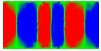
After running the simulation in "sphere_demag" the demag field can be found in "sphere.0001.gz". This file contains the "second half" of the inp file (the data section - not the finite element mesh, cf. UCD/inp Files ). In the first column there is the id of the node, for which the data are given. In the second, third, and fourth column, the Cartesian components of the magnetization are given. In the fourth column the divergence of M is given (including surface charge contributions). The fifth and sixth column give the contributions u1 and u2 to the total magnetostatic potential u, which can be found in the seventh column. In the following three columns the Cartesian components of the demagnetizing and in the next three the (combined) exchange+anisotropy field is given. The z component of the demagnetizing field is approximately Hdemag,z=-1/3 Mz, as expected for a homogeneously magnetized sphere. The x and y component should be zero, but they are not exactly zero due to numerical errors and the coarse model of the sphere. (The sphere is approximated by a polyhedron.)
The strayfield energy should be
![\[ E_\mathrm{demag}=-\frac{\mu_0}{2}\mathbf M \cdot \mathbf H_\mathrm{demag}= -\frac{\mu_0}{2}\mathbf M \cdot (-\frac{1}{3}\mathbf M)= \frac{\mu_0}{6} M_s^2 = 132629.12 \mathrm{~J/m^3} \]](form_46.png)
The simulation gives 1.311535e+05 J/m3 (see sphere.log) for the coarse model of the sphere.
We can improve the calculation by using a finer finite element mesh. This can be easily achieved by globally refining the finite element mesh. The refinement scheme implemented in magpar splits each tetrahedron into 8 smaller tetrahedra. Thus, after every refinement step we have 8 times as many elements and (approximately) 8 times as many nodes.
You can either modify the "-refine" option in allopt.txt: simulation parameters or override the setting in this file by a command line argument:
magpar.exe -refine 1
| refine | nodes | elements | Edemag (J/m3) |
|---|---|---|---|
| 0 | 849 | 3945 | 1.311535e+05 |
| 1 | 5988 | 31560 | 1.321752e+05 |
If you want to try a second refinement you will need about 300 MB of memory, because the number of nodes in the finite element mesh increases to 44919 with 5538 nodes on the boundary, which gives a boundary matrix of about 233 MB.
For the fine finite element mesh (sphere_fine.out) we find the following results:
  rm sphere.out
  ln -s ../sphere_fine.out sphere.out
  magpar.exe
  magpar.exe -refine 1
| refine | nodes | elements | Edemag (J/m3) |
|---|---|---|---|
| 0 | 2016 | 10142 | 1.318847e+05 |
| 1 | 14796 | 81136 | 1.324505e+05 |
If you want to try a second refinement you will need about 1 GB of memory, because the number of nodes in the finite element mesh increases to 113219 with 9970 nodes on the boundary, which gives a boundary matrix of about 758 MB.
sphere_larmor: Larmor precession
For the simulation of the Larmor precession the following parameters have been updated:
#########################################################################
# magpar configuration file: allopt.txt
#########################################################################

-simName sphere

-meshtype 1         # read finite element mesh from AVS inp file

-size 10e-9         # set length scaling factor to 10 nm

-init_mag 4         # start with a tilted initial magnetization

-mode 0             # select LLG time integration (PVode solver)

-demag 0            # switch off demagnetizing field

-hextini 1000       # apply a homogeneous external field of 1000 kA/m

-ts_max_time 0.03   # stop the simulation after 0.03 ns
The damping constant alpha is set to 0.0 in sphere.krn.
The simulation starts with Mx/Ms=5.773503e-01. As the magnetization precesses around the external field,Mx decreases, increases, and decreases again until it reaches its initial value again. This corresponds to one complete precession around the external field and it is completed after about 0.028435 ns.
The analytical calculation gives:
![\[ f_\mathrm{Larmor}=\frac{\gamma}{2 \pi} |H_\mathrm{ext}|= 35.176 \mathrm{~GHz} \quad, \quad \gamma=\mu_0*g*|e|/(2*m_e) = 2.210173\mathrm{e}5\mathrm{~m/As} \]](form_47.png)
![\[ \tau_\mathrm{Larmor}=1/f_\mathrm{Larmor}=0.028428477 \mathrm{~ns} \]](form_48.png)
Note, that the warning messages
...
Warning: Etot increased at t=0.0133301 ns by 1.10144e-06 (-1.90776e-12*Etot) from -577350 to -577350 J/m^3
Warning: Etot increased at t=0.0137142 ns by 2.33329e-07 (-4.04138e-13*Etot) from -577350 to -577350 J/m^3
...
indicate, that the total energy is not perfectly conserved. At every timestep there is a relative error of about 1e-12. Moreover, the magnetization does not stay perfectly homogeneous, which becomes apparent in the (slightly) increasing exchange energy.
The finite element mesh of this example has been generated using Gmsh and converted using gmsh: gmshtoucd.py (see also Preprocessing).
sphere_sw: Stoner-Wohlfarth behavior
Finally we can assume some magnetocrystalline anisotropy and calculate the switching field, if the external field is applied at different angles.
For a magnetocrystalline anisotropy constant of K1=1e5 J/m3 and Js=1 T we get an anisotropy field of Hani=2K1/Js=200 kA/m.
For this simulation the following options have been modified:
#########################################################################
# magpar configuration file: allopt.txt
#########################################################################

-simName sphere

-meshtype 0         # read finite element mesh from Patran neutral file

-size 10e-9         # set length scaling factor to 10 nm

-mode 1             # select energy minimization using TAO

-demag 0            # switch off demagnetizing field

-hextini -90.0      # apply a homogeneous external field of -90 kA/m
-htheta 0.1         # apply homogeneous external field at 0.1 rad from z-axis
-hstep -1.0         # change field amplitude in steps of -1 kA/m
-hfinal -3000       # final field value -3000 kA/m

-condinp_equil 0    # do not save output files when equilibrium is reached

-jfinal -0.1        # stop simulation if J//Hext < -0.1

-tao_fatol 0.0      # set absolute tolerance to 0 (disabled)
-tao_frtol 1e-12    # set strict relative tolerance
The results are summarized in the following graph:
sphere_cubic: Single domain particle with cubic anisotropy
In this example we can compare the anisotropy energy of a given homogeneous magnetization distribution with the analytical result. The cubic anisotropy energy is given by [1]
![\[ E_{ani}= K_1\left( m_x^2 m_y^2 + m_x^2 m_z^2 + m_y^2 m_z^2 \right) + K_2 m_x^2 m_y^2 m_z^2 = \\ \]](form_49.png)
![\[ = K_1\left( \sin^2\theta \cos^2\phi \sin^2\theta \sin^2\phi + \sin^2\theta \cos^2\phi \cos^2\theta + \sin^2\theta \sin^2\phi \cos^2\theta \right) + K_2 \sin^2\theta \cos^2\phi \sin^2\theta \sin^2\phi \cos^2\theta \]](form_50.png)
with the magnetocrystalline anisotropy constants K1 and K2.
We just change the parameter for the initial magnetization
#########################################################################
# magpar configuration file: allopt.txt
#########################################################################

-simName sphere

-meshtype 0         # read finite element mesh from Patran neutral file

-init_mag 6         # set magnetization in x-z plane to...
-init_magparm 0.785 # theta = 0.785 rad = 45 deg (from z-axis)

-demag 0            # switch off demagnetizing field
to set the magnetization in the x-z plane to a desired angle theta (defined by -init_magparm measured from the z-axis). It is assumed that the axes of the cubic lattice coincide with Cartesian coordinate system (theta=phi=psi=0). In general the cubic axes are defined by the Euler angles in project.krn: material properties.[2,3]
The run script completes a series of 20 simulations which vary the angle theta between 0 and 180 deg. The following figure shows the results for K1=4.6e5 J/m3, K2=1.5e4 J/m3, which are in perfect agreement with the analytical calculation.
[1] L. W. McKeehan, "Ferromagnetic Anisotropy in Nickel-Cobalt-Iron Crystals at Various Temperatures", Phys. Rev. 51 (1937) 136-139. [2] Eric W. Weisstein. Euler Angles. From MathWorld - A Wolfram Web Resource.
[3] Euler angles in Wikipedia.
iface: Domain wall pinning
For yet another problem, we have an analytical result to compare with: The pinning field of a Bloch wall at a perfect planar interface (e.g. a grain boundary). The analytical solution can be found in Ref. [4].
They find:
![\[ H_\mathrm{pin}= \frac{2 K^{\mathrm{II}}_1}{J_\mathrm{s}^\mathrm{II}} \frac{1-\varepsilon_A \varepsilon_K} {(1+\sqrt{\varepsilon_A \varepsilon_J})^2} \quad , \]](form_51.png)
where
![\[ \varepsilon_J = \frac{J_\mathrm{s}^\mathrm{I}}{J_\mathrm{s}^\mathrm{II}} \quad , \quad \varepsilon_A = \frac{A^\mathrm{I}}{A^{\mathrm{II}}} \quad , \quad \varepsilon_K = \frac{K^\mathrm{I}_1}{K^{\mathrm{II}}_1} \quad \]](form_52.png)
and (I) denotes the material parameters of the softer material and (II) those of the harder material.
The simulation is initialized with a domain wall and an external field moves the domain wall towards the interface, where it gets pinned. As the external field increases the Bloch wall is more and more forced into the "harder material" until it depins and propagates further through the "harder material".
This example consists of
- allopt.txt: simulation parameters
- iface.gid
the GiD model - iface.inp
the INP file, which has been generated by GiD - iface.krn
material parameters: Sm2Co17 and SmCo5 - run
shell script to run magpar (not required)
For the material parameters given in iface.krn, the analytical formulas above give a pinning field of Hpin=1933 kA/m.
#########################################################################
# magpar configuration file: allopt.txt
#########################################################################

-simName iface

-refine 2           # refine mesh 2 times

-size 13e-9         # set length scaling factor to 13 nm

-init_mag -9        # initialize magnetization with Bloch wall and reverse
-init_magparm 0.7

-mode 1             # select energy minimization using TAO

-demag 0            # switch off demagnetizing field

-hextini -1700      # apply a homogeneous external field of 12 kA/m
-hstep   -5         # change field amplitude in steps of -5 kA/m
-hfinal  -5000      # final field value -5000 kA/m

-condinp_equil 0    # do not save output files when equilibrium is reached
-condinp_t  1e99    # do not save output files at regular time intervals

-slice_n 0,0,1      # slice plane for png files: x-y-plane
-slice_p 0,0,0.5

-line_v 1,0,0       # set measurement line parallel to x-axis
-line_p 0,0.5,0.5

-logpid 1           # save average magnetization in output files (*.log_XXX)

-tao_fatol 1e-10    # set absolute tolerance for energy minimizer TAO
-tao_frtol 1e-10    # set relative tolerance for energy minimizer TAO
The "run" script automatically varies the mesh density using the "-refine" option. It runs three simulations starting with a very coarse mesh, which is refined once and twice in the following runs. One can observe, that the simulation result gets closer to the analytical result as the mesh density increases.
[4] H. Kronmüller, D. Goll, "Micromagnetic theory of the pinning of domain walls at phase boundaries", Physica B: Condensed Matter, 319 (2002) 122-126.
mumag3: mumag standard problem #3
mumag standard problem #3 asks to calculate the single domain limit of a cubic magnetic particle. For a certain size L the total energy of the so-called flower state on the one hand, and the vortex or curling state on the other hand is equal. The material parameters have been chosen according to the definition on the mumag website. Just the anisotropy axis has been rotated by 90 deg into the x-axis to make the initialization of the vortex state easier.
With Ms=1 T and A=1e-11 J/m we find Km=1/2*mu0*Ms2=3.9788736e5 and set K1=0.1*Km=3.9788736e4 J/m3. lex=(A/Km)1/2=5.013256 nm.
#########################################################################
# magpar configuration file: allopt.txt
#########################################################################

-simName mumag3

-meshtype 0         # read finite element mesh from Patran neutral file

-refine 4           # refine mesh 4 times

-size 30e-9         # set length scaling factor to 30 nm

-init_mag 1         # initialize magnetization parallel to x-axis

-mode 1             # select energy minimization using TAO

-slice_n 0,0,1      # slice plane for png files: x-y-plane
-slice_p 0,0,0

-line_v 0,0,1       # set measurement line parallel to z-axis
-line_p 0,0,0

-tao_fatol 1e-8     # set absolute tolerance for energy minimizer TAO
-tao_frtol 0.0      # set relative tolerance for energy minimizer TAO
In this example we use the global refinement feature of magpar. The neutral file "mumag3.out" describes a very simple finite element discretization of a cube with 8 nodes and 5 tetrahedral finite elements. The option "-refine 4" makes magpar refine this mesh 4 times, which gives 5*84=5*4096=20480 elements and 4233 nodes.
The shell script "run" should be used to run this example. It takes advantage of some useful features of magpar (rather PETSc) to run several simulations with different parameters in one go:
It contains two loops. One which selects the initial magnetization:
-init_mag 1
homogeneous magnetization in x-direction-init_mag 7
approximate flower state
And another loop which varies the size of the cube from 30 nm to 50 nm.
magpar is then called with the command line options "-init_mag" and "-size", which override the settings in the allopt.txt: simulation parameters configuration file. All simulations append their results to the existing "mumag3.log" file. In order to store the setting of the initial magnetization and size a simple echo command adds some comment lines to the log file just before a new simulation is started.
Finally, one just has to extract the settings of the size and total energy in equilibrium to create a plot, which shows the total energy as a function of size for flower and vortex state. With the parameters in this example we find the following result:
mumag3b: mumag standard problem #3 with 2 cubes
This example is very similar to the previous example mumag3: mumag standard problem #3. However, in this example the geometry consists of two disjoint cubes, where the material parameters of one are set to air/vacuum, while the other one is magnetic.
  0.0       0 0.0         0.0  0.0  0.0      0.1   uni    # cube1: air
  1.5707963 0 3.9788736e4 0.0  1.00 1.00E-11 0.1   uni    # cube2: mumag standard problem #3 http://www.ctcms.nist.gov/~rdm/mumag.html
#
# theta phi   K1       K2      Js   A        alpha psi    # parameter
# (rad) (rad) (J/m^3)  (J/m^3) (T)  (J/m)    (1)   (rad)  # units
The geometry and finite element mesh of this example have been generated with Gmsh and converted with gmsh: gmshtoucd.py (see Preprocessing).
This example also demonstrates the use of the option "-logpid 1" in allopt.txt and how non magnetic volumes can be included in simulations with magpar (e.g. to calculate the magnetostatic field surrounding a magnet).
nanodot: Nanodot
In case a simulation was interrupted or it should be continued at a certain point, it can be restarted from any UCD file (project.INP.gz).
For example, we restart the simulation of the magnetization reversal of a magnetic nanodot.
We need the following files:
- allopt.txt: simulation parameters
- run
shell script to run magpar (not required) - nanodot.krn
material parameters: permalloy - nanodot.0050.inp
UCD file with the magnetization distribution of some magnetization state in a positive field - nanodot.inp
UCD file with the finite element mesh
The UCD file with the magnetization distribution has to be created from a previous simulation run. First one has to search the project.log file of the old simulation for the correct number of the UCD file (e.g., search the fourth column where Hext==12 and the first column where eq==1 to find the equilibrium state in a field of 12 kA/m). If an inp file has been written, its number can be found in the second column. Otherwise one has to take some other inp number nearby.
Then, a full UCD file is created using the mkinp.sh shell script (cf. UCD/inp Files).
mkinp.sh nanodot.0001.femsh nandot.0050.gz
As a result, the file nanodot.0050.inp is created.
Since this UCD file also contains the full geometry of the finite element mesh, it can also be used for the nanodot.inp file. A simple copy
cp nanodot.0050.inp nanodot.inp
or a symbolic link (which saves some disk space)
ln -s nanodot.0050.inp nanodot.inp
should work.
However, it should be noted, that the original UCD files (generated with GiD) or neutral files (generated with Patran) cannot be used for the nanodot.inp file, if the simulation has been run in parallel. The reason is, that the nodes of the finite element mesh are renumbered after mesh partitioning. Thus, the numbering of the nodes in the output files is different from the numbering in the original UCD or neutral file! Therefore, any time a simulation is restarted (continued), the mesh has to be read from the same UCD file, from which the magnetization distribution is read.
Finally, the simulation parameters in allopt.txt: simulation parameters have to be updated:
#########################################################################
# magpar configuration file: allopt.txt
#########################################################################

-simName nanodot

-size 100e-9        # set length scaling factor to 100 nm

-init_mag 0         # read magnetization from inp file with...

-inp 0059           # ...inp number 0059

-mode 0             # select LLG time integration (PVode solver)

-hextini 32         # apply a homogeneous external field
-htheta  1.5707963  # apply homogeneous external field parallel to x-axis
-hstep   -5         # change field amplitude in steps of -5 kA/m
-hfinal  -200       # final field value -200 kA/m

-condinp_j  0.05    # save output files when J//Hext changes by 0.05
-condinp_t  1e99    # do not save output files at regular time intervals

-slice_n 0,0,1      # slice plane for png files: x-y-plane
-slice_p 0,0,0.1

-jfinal -0.2        # stop simulation if |J//Hext| < jfinal

-ts_max_time 1e99   # effectively disable maximum simulation time
Then, the simulation can be restarted.
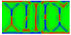
The simulation parameters have been set to calculate the demagnetization curve of a magnetic nanodot. At the nucleation field (still a positive field!) a magnetic vortex structure nucleates on the boundary of the nanodot and quickly moves towards the center (it really precesses depending on the damping parameter!). As the external field is reduced, the vortex moves towards the boundary again until it is annihilated.
Section Postprocessing presents some tools to visualize the results of the simulation, which are quite pretty and colorful.
More details about the properties of magnetic nanodots can be found in the following paper:
W. Scholz, K. Y. Guslienko, V. Novosad, D. Suess, T. Schrefl, R. W. Chantrell, J. Fidler,
"Transition from single-domain to vortex state in soft magnetic cylindrical nanodots",
J. Magn. Magn. Mater. 266 (2003) 155-163.
A preprint is available here.
nanodot_demag: Nanodot demag energy
This simple example just calculates the magnetostatic field and energy of a homogenneously magnetized cylinder (nanodot).
The configuration file is very short since we can use the default settings of all other options.
#########################################################################
# magpar configuration file: allopt.txt
#########################################################################

-simName nanodot

-size 100e-9         # set length scaling factor to 100 nm

# Du-Xing Chen, James A. Brug, and Ronald B. Goldfarb,
# "Demagnetizing Factors for Cylinders,"
# IEEE Trans. Magn. 21 (1991) 3601-3619.
# http://dx.doi.org/10.1109/20.102932
#
# p. 3604, Tab. 1
#
# gamma   N_m
# --------------
# 0.10    0.7967
#
# gamma ... dot aspect ratio (thickness/diameter)
# N_m   ... demagnetizing factor
#
# E_dem=0.7967/2*M_s^2*mu_0=0.39835*mu_0=316997 J/m^3
#
# more values from Table 1 in the paper cited above:
#
# gamma   N_m         gamma   N_m         gamma   N_m
# --------------      --------------      --------------
# 0.00001 0.9999      0.26    0.6262      1.4     0.2429
# 0.0001  0.9994      0.28    0.6101      1.6     0.2186
# 0.001   0.9950      0.30    0.5947      1.8     0.1986
# 0.01    0.9650      0.32    0.5801      2.0     0.1819
# 0.02    0.9389      0.34    0.5662      2.5     0.1501
# 0.03    0.9161      0.36    0.5530      3.0     0.1278
# 0.04    0.8954      0.38    0.5403      3.5     0.1112
# 0.05    0.8764      0.40    0.5281      4       0.09835
# 0.06    0.8586      0.45    0.4999      5       0.07991
# 0.07    0.8419      0.50    0.4745      6       0.06728
# 0.08    0.8261      0.55    0.4514      7       0.05809
# 0.09    0.8110      0.60    0.4303      8       0.05110
# 0.10    0.7967      0.65    0.4110      9       0.04562
# 0.12    0.7698      0.70    0.3933      10      0.04119
# 0.14    0.7450      0.75    0.3770      20      0.02091
# 0.16    0.7219      0.80    0.3619      50      0.008438
# 0.18    0.7004      0.90    0.3349      100     0.004232
# 0.20    0.6802      1.0     0.3116      200     0.002119
# 0.22    0.6611      1.1     0.2911      500     0.0008483
# 0.24    0.6432      1.2     0.2731      1000    0.0004243
The result of the simulation can be compared with the analytical result given in the allopt.txt file above. With the given FE mesh we obtain a pretty good result (3.158828e+05 J/m^3: error of -0.6%), with one refinement the result is even closer (3.166590e+05 J/m^3: error of -0.1%).
stress: Magnetoelastic effects on domain structure
Ahmet Kaya from the research group of Jim Bain and Jimmy Zhu at the Data Storage Systems Center (DSSC) at Carnegie Mellon University implemented magnetoelastic/magnetostriction effects in magpar based on the following papers:
Daniel Z. Bai, Jian-Gang Zhu, Winnie Yu, and James A. Bain
Micromagnetic simulation of effect of stress-induced anisotropy in soft magnetic thin films
Journal of Applied Physics, Volume 95, Number 11, June 2004, pp. 6864-6866
[ J. Appl. Phys. 1 ] [ J. Appl. Phys. 2 ]
Daniel Bai,
Micromagnetic Modeling of Write Heads for High-Density and High-Data-Rate Perpendicular Recording
dissertation, Department of Electrical and Computer Engineering, Carnegie Mellon University, Aug. 2004.
This example uses material parameters typical of Fe65Co35 (Ms=2.4 T) and random texture (as defined in the project.kst: magnetoelastic properties file stress.kst).
  7        17.5e-6   103.7e-6  -1e9    0.0     0.0      # Fe65Co35: Bai, J. Appl. Phys. 95 (2004) 6864-6866.
#
# texture  lamda100  lamda111  sigmaX  sigmaY  sigmaZ   # parameter
# (-)      (erg/cm^3)(erg/cm^3)(Pa)    (Pa)    (Pa)     # units
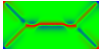
The example reproduces the results shown in Fig. 2 in the paper. It is interesting to compare with the zero stress case, which gives the classic closure domain pattern. FIXME: requires fine mesh with -refine 1 !!!
#########################################################################
# magpar configuration file: allopt.txt
#########################################################################

-simName stress

-size 1e-6          # set length scaling factor to microns

-init_mag 0         # read magnetization from inp file with...

-inp 0002           # ...inp number 0002 (stress.0002.inp)

-mode 0             # select LLG time integration (PVode solver)

-htheta 1.5707963   # set htheta to measure J//Hext parallel to x-axis

#-helastic_propfile stress.kst  # read magnetoelastic material parameters from file

-slice_n 0,0,1      # slice plane for png files: x-y-plane
-slice_p 0,0,0.04

-ts_max_time 9.0    # stop the simulation after 9 ns
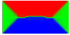
Equilibrium domain structure with magnetoelastic effects (1 GPa compressive stress in x-direction with random texture):
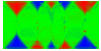
x-direction: parallel to the long axis
y-direction: parallel to the short axis
z-direction: perpendicular to the thin film
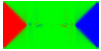
Without magnetoelastic effects:
Another interesting reference:
Pei Zou, Winnie Yu, and James A. Bain,
Influence of Stress and Texture on Soft Magnetic Properties of Thin Films
IEEE Trans. Magn. 38 (2002) 3501-3520.
[ IEEE Trans. Magn. 1 ] [ IEEE Trans. Magn. 2 ]
thinfilm: Thin magnetic film
The calculation of the demagnetizing factor of a thin magnetic film is shown in this example. A thin film of infinite size (in the plane) has a demagnetizing factor of Dz=1. However, for a small platelet of finite size (1000 x1000 x50) the demagnetizing factor is smaller (Dz < 1) and we can calculate its value analytically using Rok Dittrich's Calculator for magnetostatic energy and demagnetizing factor. For the given aspect ratio, a material with a saturation magnetization of 1 T and a homogeneous magnetization distribution perpendicular to the plane we find Dz=0.881 and a magnetostatic energy density of E=350.54 kJ/m3.
#########################################################################
# magpar configuration file: allopt.txt
#########################################################################

-simName thinfilm

-size 1e-6          # set length scaling factor to microns

-slice_n 0,0,1      # slice plane for png files: x-y-plane
-slice_p 0,0,0.025
The numerical simulation with magpar gives for different refinement levels (using the "-refine" option):
| refine | nodes | elements | boundary matrix | Edemag (J/m3) |
|---|---|---|---|---|
| 0 | 1014 | 2974 | < 1MB | 3.444659e+05 |
| 1 | 5962 | 23792 | 89 MB | 3.486828e+05 |
| 2 | 39559 | 190336 | 1801 MB | 3.499780e+05 |
The simulation of models with a very flat geometry requires lots of memory because the size of the boundary matrix, which is required for the calculation of the demagnetizing field, scales quadratically with the number of nodes on the surface.
Running a simulation in parallel
In order to run a simulation in parallel on a multiprocessor machine, it is sufficient to set the variable "np" in the "run" scripts to any desired number of processes. This can also be tested on single processor machines, where the processes have to share a single CPU. Of course, this is not very efficient but very useful during development and debugging!
On workstation clusters the proper invocation of parallel programs depends on the local configuration. Usually, there is a job queueing system installed, which takes care of the scheduling and distribution. Most queueing systems support the execution of parallel jobs. Please, ask the system administrator of your machine how to run MPI jobs.
MPI usually requires a machine-file, which contains a simple list of possible machines to run on (e.g. machines.txt). These machines must be accessible by rlogin or ssh without a password (cf. section MPI).
To run magpar.exe on 10 processors distributed over the machines listed in machines.txt:
MPICH1 syntax:
mpirun -machinefile machines.txt -np 10 magpar.exe
MPICH2 syntax:
  # create file with secret passphrase (change "mysecret")
  echo "MPD_SECRETWORD=mysecret" > ~/.mpd.conf
  chmod 600 ~/.mpd.conf
  # create list of available machines
  cp machines.txt mpd.hosts
  # start daemons on 3 machines on (some of) the hosts in mpd.hosts
  mpdboot -n 3
  # check that all daemons are up and running
  mpdtrace; mpdringtest 100
  mpiexec -l -n 3 magpar.exe
LAM/MPI syntax:
  $LAMBIN/lamboot machines.txt
  $LAMBIN/mpirun -c 10 magpar.exe
  $LAMBIN/lamhalt